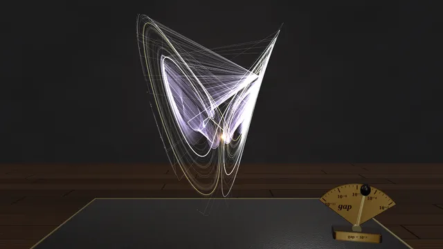
Lorenz Attractor
Drop probe clouds into the butterfly of chaos and watch them part.
How to play
- Tap anywhere in the dark space around the butterfly to drop a cloud of probe particles there, and watch the flow pull them in.
- Drag the bright state point to a new spot. Its neighbours gather under your finger; let go and watch them spread apart.
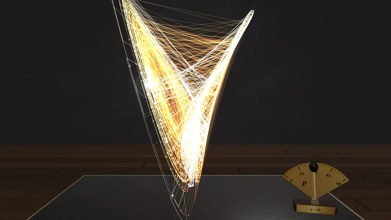
- Pull the brass ρ lever on the plinth to heat the convection harder or more gently. Below about 24 the chaos dies away.
- Drag empty space to turn the view. Try the three Challenges, or open Lab for σ, β and the presets.
Challenges
- Tap the dark space beside the butterfly and watch the probe cloud get pulled onto it
- Drag the bright state point, let go, and watch its neighbours spread over both wings
- Pull the ρ lever below 24 and let the chaos settle onto two still points
Try this
- Lower ρ (rho) to 15. The swarm stops wandering and spirals into two still points, one in each wing.
- Push ρ up to 160. The chaos gives way to a single repeating loop, and the chaos rate drops to almost zero.
- Return to the classic values and wait for λ to settle near 0.9: each time unit, a tiny error grows by a factor of about e^0.9 ≈ 2.5.
Fun facts
- Edward Lorenz published these equations in 1963 in a paper titled “Deterministic Nonperiodic Flow”.
- Lorenz noticed the sensitivity when he restarted a weather simulation from numbers rounded to three decimal places, and the forecast soon came out completely different.
- In 2002 Warwick Tucker proved by a computer-assisted proof that the Lorenz attractor really exists, solving the 14th of Stephen Smale’s problems for the 21st century.
- At the classic values, nearby paths separate at a rate of about 0.9 per time unit, the system’s largest Lyapunov exponent.
Order inside chaos
In 1963 the meteorologist Edward Lorenz boiled a model of air rising and falling in a heated layer down to just three equations. The variable x measures how fast the convection roll turns, y the temperature difference between rising and sinking air, and z how far the temperature profile is bent away from a straight line:
dx/dt = σ(y − x), dy/dt = x(ρ − z) − y, dz/dt = xy − βz.
The equations contain no randomness at all, yet their solutions never settle down and never repeat. Each particle here is one possible state of the system, moving according to the equations. Start them anywhere and they are drawn onto the same twisted two-winged shape, the Lorenz attractor. It is called strange because it is a fractal: zoom in on what looks like a single sheet and you find layers within layers.
What the knobs do
σ (sigma, the Prandtl number) compares how quickly the fluid’s motion and its heat spread through it, β (beta) relates to the shape of the convection cell, and ρ (rho) is how strongly the layer is heated. With gentle heating (ρ below 1) nothing moves. Above that, the fluid rolls steadily, and the swarm settles onto one of two still points, one in each wing. Around ρ ≈ 24.74 those steady states become unstable and the classic chaotic butterfly appears. At much larger ρ, such as 160, the motion locks into a single repeating loop. We checked each preset numerically.
Measuring chaos
The “Chaos rate λ” readout follows one particle and an invisible twin that starts 10⁻⁸ away. After every few steps it measures how much their gap has grown, adds up the logarithms and pulls the twin back. The average growth rate is the largest Lyapunov exponent. For the classic values it settles near 0.9 per time unit, matching the published value of about 0.906. A negative value means the swarm is converging, as at ρ = 15.
Shrinking volumes
The Lorenz flow is dissipative: any blob of starting states shrinks in volume by a factor e^(−(σ + 1 + β)t), about 13.7 e-foldings per time unit at the classic values. That is why every starting point ends up on a thin attractor with no volume, even though it is infinitely long.
For the curious
Every particle is advanced with the classical fourth-order Runge–Kutta method in fixed steps of 0.004 time units, independent of your screen’s frame rate. Trails are sampled at equal intervals of model time, and particles start on the attractor itself, taken from one long warmed-up trajectory. The steady states sit at x = y = ±√(β(ρ − 1)), z = ρ − 1.
Questions people ask
What is the Lorenz attractor?
The set of states that the three Lorenz equations settle onto. Every path is pulled onto a two-winged butterfly-shaped surface and then wanders round it forever without repeating.
Why is the Lorenz system chaotic?
The flow stretches nearby states apart and folds them back onto the attractor. Repeated stretching makes tiny differences grow exponentially, so long-term predictions become impossible.
What do σ, ρ and β mean?
They come from Lorenz’s model of convection: σ relates to the fluid’s viscosity and heat conduction, ρ to how strongly the fluid is heated, and β to the shape of the convection cell.